Powder Charge Testing

ChronoPlotter supports creating graphs comparing charge weight and velocity.

Table of contents:

• Importing chronograph files (LabRadar, MagnetoSpeed, ProChrono)
• Round-Robin (OCW) and Satterlee testing
• Manually entering velocity data

Importing chronograph files

If your data is recorded on an SD card (for instance with LabRadar or MagnetoSpeed V3), make sure it’s plugged into your computer.

• For LabRadar: Click the Select LabRadar directory button, navigate to your SD card, and click Select Folder to confirm.
• For MagnetoSpeed: Click the Select MangetoSpeed file button, navigate to your SD card, and select the LOG.CSV file.
• For ProChrono: Click the Select ProChrono file button and select your CSV file.
• If your chronograph doesn’t save or export data to a file, click the Manual data entry button to enter your velocity data manually.

The following example shows a LabRadar SD card:

The program should now be populated with all of your recorded data:

Uncheck any series you don’t want to include in the graph. Then enter a charge weight for each series, or click the Auto-fill charge weights button to automate the process:

To include details in the graph about the components used in testing, additionally fill in the text fields on the right:

Clicking Show graph pops open a new window with a preview of the generated graph. Note: This does not save your graph, only displays it.

The graph will look something like this:

You can alternatively create a line chart with standard deviation error bars by selecting it from the Graph type drop-down.

By default, ChronoPlotter displays ES (Extreme Spread), SD (Standard Deviation), and the series-to-series difference in velocity for each series in the graph. The average (mean) velocity for each series can also be displayed but is unchecked by default. You can add, remove, or change the location of these details in the graph under the Graph options section.

Close the preview window, making sure not to close ChronoPlotter itself. Finally, click Save graph as image to save your graph as a .PNG, .JPG, or .PDF file.

Round-Robin (OCW) and Satterlee testing

ChronoPlotter supports chronograph data recorded using the “round-robin” method popular with OCW testing. First, uncheck any series not part of the round-robin:

Click Convert from round-robin to open this dialog:

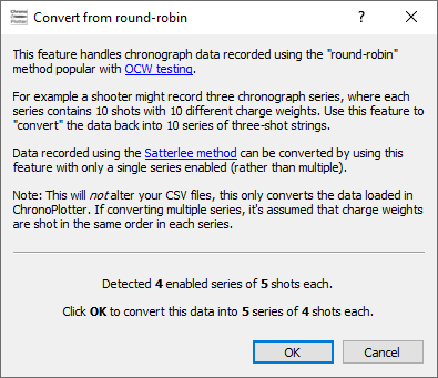
Then click OK to convert the series data into traditional series suitable for graphing. Note that ChronoPlotter does not alter your CSV files, this only converts the data loaded in the program:

Likewise, this same feature can be used to convert data recorded using the Satterlee method. This is because at its core Satterlee is simply a “one shot round-robin” test. To do so, uncheck all other series except for the one series containing Satterlee data, then click Convert from round-robin and proceed as usual.

Thanks to TallMikeSTL for contributing test data.

Manual data entry

Begin by clicking the Manual data entry button:

By default, a single empty series is created. Click the Add new series button to create additional series for each charge weight being tested. Then enter a charge weight for each series, or click the Auto-fill charge weights button to automate the process:

To enter velocity data for a series, click the Enter velocity data button, enter each number on a new line, and click OK:

To include details in the graph about the components used in testing, additionally fill in the text fields on the right:

Clicking Show graph pops open a new window with a preview of the generated graph. Note: This does not save your graph, only displays it.

The graph will look something like this:

Close the preview window, making sure not to close ChronoPlotter itself. Finally, click Save graph as image to save your graph as a .PNG, .JPG, or .PDF file.